Choosing the “right” demand forecasting model

Tailoring model selection

Say you sell a machine as well as parts and supplies for that machine. Think razor and razor blades, or coffee maker and coffee pods. What demand looks like for each of these categories is probably pretty different, necessitating different algorithms. Say you further sell coffee pods with seasonal flavors in addition to your base flavors. Demand for these SKUs probably looks different too, again making different algorithms the best for each one.

The right one could also change over time. Naturally, as a product goes through its lifecycle demand patterns will shift. But it could also be the result of changes you make. For example, you might switch from doing frequent promotions to an “everyday low price” marketing strategy. This shift will likely make a different algorithm the best one for your products.

Even with today’s computing power, we don’t recommend blindly throwing every algorithm at the problem to see what emerges as the “winner.” For one, it can become a distraction. Your team gets caught up adding algorithms when they should be focused on adjusting plans based on the latest data. For another, it leads to a lack of transparency and understanding of how a forecast was created. That makes it hard to explain your demand plan, and even harder to build trust in it.

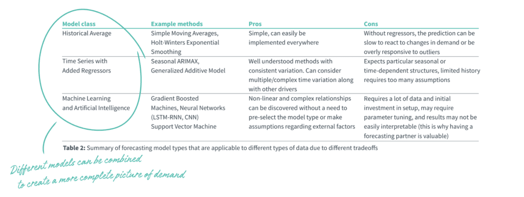
Instead, make educated decisions about which models are right for each of your products based on their characteristics, aided by technology as much as possible. Next we’ll review three different classes of commonly used modeling methods and their associated tradeoffs.

1. Historical average

Historical average models smooth out demand by taking averages over different historical periods. This is one of the simplest classes of forecasting models and tends to work well for long-term or high-level demand planning, where basic trends over time are most important to understand and the daily or weekly variation can be de-emphasized.

• Pros: The primary advantage of a historical average model over other methodologies is its simplicity; you can easily implement this type of model with almost any tool, including Excel and Tableau. That makes it relatively easy to compare results in different systems or debug calculation errors.
• Cons: Historical averages are anchored to their previous periods and react to changes slowly. If demand has changed significantly over the past month, or even the past year, the trend won’t be fully captured in your forecast. Conversely, they are also overly responsive to outliers in the data because they do not use regressors. A single spike or dip can have an outsized influence on your forecast.
• Example model types:Simple Moving Averages, Holt-Winters Exponential Smoothing, Optimized Theta
• Best for:Products with low forecastability. These products may be regularly sold, but have low daily/weekly volume. As a result, intermittent demand is hard to predict and improving the forecast doesn’t add a lot of value. You can also use these methods for high-level budgeting and planning, since they smooth out short-term and seasonal variations.

2. Time series with added regressors

This class features regression models that are fit by comparing different historical time periods. These models can also incorporate other inputs, such as price promotions, seasonality and weather patterns.

• Pros: Models in this class are especially adept at predicting products that have consistent variation, such as established seasonality trends. These models can also take into account additional factors known to influence demand, such as promotional and price activity.
• Cons: Regression models expect consistent variation in the data, which means that datasets with a limited history force the model to make a fit on too few data points. You must inspect the time series for proper assumptions, such as stationarity and homoscedasticity. You also need to scale and pre-select regressors to prevent issues like multicollinearity.
• Example model types: Seasonal ARIMA, Generalized Additive Models (GAM), Bayesian Structural Time Series (BSTS), TBATS
• Best for: Products with well-defined seasonality or changes in demand, e.g., swimsuits and winter coats, and products for which the effects of promotional activity can be easily captured using regressors.

3. Machine Learning/Artificial Intelligence

Machine learning models are a broad set of methodologies that use more complex mathematical techniques to select variables and optimize fit where there may be complicated interactions between features. These can be powerful choices, but you’ll want to make sure these obey the integrated, transparent and actionable properties described in our white paper.

• Pros: These types of models are great for discovering non-linear and complex relationships in your data, without needing to preselect the exact model type or make assumptions about external factors. Instead of explicitly weighting variables or variable interactions, many of these methods allow you to determine variable importance without worrying about the effects of multicollinearity.
• Cons: The challenge with machine learning is it requires a lot of input data and a fair amount of investment in setup and maintenance. The results of these types of models can also be more complicated to interpret correctly and can be prone to overfitting.
• Example model types: Neural Networks (FFNN, LSTM-RNN, CNN), Random Forest, Gradient Boosted Machines, Support Vector Machine
• Best for: Products sold widely and very frequently that may have nuanced buying patterns given the scope and volume of sales.

Which model is best?

While the increased complexity of AI/ML models can yield more accurate demand forecasts in some cases, tradeoffs in the difficulty of implementation mean that the nuances of your products determine which model will yield the best results for you. So, how do you go about choosing the right model, or set of models, for your business?

Weighing each model’s pros and cons is a start, but your products might not neatly fit into a single type. To work around this limitation, it’s also possible to build an ensemble model. This approach takes models from multiple different classes and averages across them. It has the benefit of incorporating effects generated from each methodology, strengthening similar effects while canceling out inconsistent effects.